Conditional Gaussian KDE

Here we go through a simple example of a conditional Gaussian KDE. Let’s imagine we would like to sample from the distribution \(P(x|y)\), given that samples from a full distribution \(P(x, y)\) are available. Example of such scenario could be an MCMC chain, fitted for both \(x\) and \(y\).

In general, such procedure is not possible as one would need to run MCMC from beginning, by sampling \(P(x|y)\) directly, for one particular \(y\). However, if we make an analytical form of the total pdf, then in principle we could obtain such conditional distribution for any \(y\).

ConditionalGaussianKernelDensity class implements these functionalities:

• fitting the Gaussian KDE for the total distribution \(P(x, y)\) form its samples,

• slicing through it to either obtain samples of the \(P(x | y)\), or calculate the exact values of the conditional probability.

%matplotlib inline
%load_ext autoreload
%autoreload 2
import numpy as np
import matplotlib.pyplot as plt
plt.rc('text', usetex=True)
plt.rc('font', family='serif')

from conditional_kde import ConditionalGaussianKernelDensity

As an example, let’s create a simple 2D sample of points and fit KDE with it.

mean1, cov1 = [0, -5], [[1, 0], [0, 5]]
mean2, cov2 = [10, 5], [[5, 0], [0, 1]]
data_xy = np.concatenate(
    (
        np.random.multivariate_normal(mean1, cov1, 10000),
        np.random.multivariate_normal(mean2, cov2, 10000)
    ),
    axis = 0
)
data_y = data_xy[:, 1, np.newaxis]
plt.figure(figsize = (5, 5))
plt.hist2d(data_xy[:, 0], data_xy[:, 1], bins = 50)
plt.xlabel("$x$", fontsize = 20)
plt.ylabel("$y$", fontsize = 20);

Two most important parameters of the KDE are whitening_algorithm and bandwidth. Whitening is the process of normalizing the data in some way, here we implement three different ones:

• None - no normalization

• "rescale" - rescaling every dimension to be of unit-variance

• "ZCA" - whitening along principal component axes

Bandwidth on the other hand controls the size of Gaussians around each point. Higher bandwidth will give wider and smoother distributions. We implement several ways of choosing its value:

• "scott" - uses approximate relation depending on the number of samples and dimensions - Scott’s parameter

• "optimized" - searches for the best bandwidth by minimizing KL divergence between real distribution samples and fitted KDE

Besides that, we allow to specify its value explicitly.

kde = ConditionalGaussianKernelDensity(
    whitening_algorithm = "rescale",
    bandwidth = "optimized",
    steps = 10,
    cv_fold = 5,
    n_jobs = -1,
    verbose = 1,
)
kde = kde.fit(
    data_xy,
    features = ["x", "y"],
)

Fitting 5 folds for each of 10 candidates, totalling 50 fits

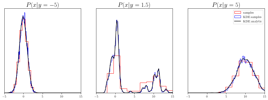
Now we can either pull samples for some conditional values of y, or calculate analytical distributions for it.

mini, maxi = -5, 15
X = np.linspace(mini, maxi, 100)
fig, axes = plt.subplots(1, 3, sharey = True, figsize = (15, 5))
epsilon = 2.0
for y, ax in zip([-5, 1.5, 5], axes):
    # plotting histogram of actual samples
    ax.hist(
        data_xy[
            np.logical_and(
                data_xy[:, 1] > y - epsilon / 2,
                data_xy[:, 1] < y + epsilon / 2,
            ),
            0
        ],
        # bins = 100,
        density = True,
        label = "samples",
        histtype = "step",
        color = "red",
    )
    # pulling conditional samples
    data_x_cond_y = kde.sample(
        conditionals = {"y": y},
        n_samples = 10000,
        keep_dims = False,
    )
    # plotting histogram
    ax.hist(
        data_x_cond_y,
        bins = 100,
        density = True,
        label = "KDE samples",
        histtype = "step",
        color = "blue",
    )

    # calculating analytical probabilities along the axis
    x = np.stack([X, np.ones(len(X)) * y], axis = -1)
    probs = np.exp(kde.score_samples(x, conditional_features = ["y"]))
    # plotting the function
    ax.plot(X, probs, label = "KDE analytic", color = "black")

    ax.set_title(f"$P(x | y = {y})$", fontsize = 20)
    ax.set_xlim((mini, maxi))
    ax.set_yticks([])
    ax.set_xticks([-5, 0, 5, 10, 15])
plt.legend();

ZCA whitening

Instead of a simple rescale of dimensions, potentially more powerful whitening can be obtained with ZCA algorithm. It scales the data along the principal axis. The method comes with a bit bigger computational overhead. Here we show results for the same example as before.

kde = ConditionalGaussianKernelDensity(
    whitening_algorithm = "ZCA",
    bandwidth = "optimized",
)
kde = kde.fit(
    data_xy,
    features = ["x", "y"],
)

mini, maxi = -5, 15
X = np.linspace(mini, maxi, 100)
fig, axes = plt.subplots(1, 3, sharey = True, figsize = (15, 5))
epsilon = 2.0
for y, ax in zip([-5, 1.5, 5], axes):
    # plotting histogram of actual samples
    ax.hist(
        data_xy[
            np.logical_and(
                data_xy[:, 1] > y - epsilon / 2,
                data_xy[:, 1] < y + epsilon / 2,
            ),
            0
        ],
        # bins = 100,
        density = True,
        label = "samples",
        histtype = "step",
        color = "red",
    )
    # pulling conditional samples
    data_x_cond_y = kde.sample(
        conditionals = {"y": y},
        n_samples = 10000,
        keep_dims = False,
    )
    # plotting histogram
    ax.hist(
        data_x_cond_y,
        bins = 100,
        density = True,
        label = "KDE samples",
        histtype = "step",
        color = "blue",
    )

    # calculating analytical probabilities along the axis
    x = np.stack([X, np.ones(len(X)) * y], axis = -1)
    probs = np.exp(kde.score_samples(x, conditional_features = ["y"]))
    # plotting the function
    ax.plot(X, probs, label = "KDE analytic", alpha = 0.7, color = "black")

    ax.set_title(f"$P(x | y = {y})$", fontsize = 20)
    ax.set_xlim((mini, maxi))
    ax.set_yticks([])
    ax.set_xticks([-5, 0, 5, 10, 15])
plt.legend();